<< Click to Display Table of Contents >> Navigation:  User DLLs > Add-In DLLs > Extra DLLs > Profile Rate of Change (dcu_formTl.dll)

 

Overview

All systems, whether mechanical, electrical, informational or otherwise have certain common properties. One of these properties is that the input includes noise, as well as the desired input. The system process filters the noise, and since no process is perfect there is always an element of distortion as well. Distortion is highly process specific and is beyond the scope of this paper. This paper will focus on the filtering of the input noise.

 

The rate at which the output can change in response to an input imposes a limit on how much noise is transmitted through the system. Noise is composed of a combination of sinusoids at different frequencies and phases. For many physical systems, the high frequency components of the noise change at a rate that exceeds the response time of the system, and therefore cannot be transmitted through the system. Lower frequency components are transmitted to the output because they change slowly enough so that the system can respond to them.

 

A good illustration of this is a car with sloppy steering. If the driver whips the steering wheel back and forth quickly the car does not radically change direction because the response time of the steering is slow. However, gentle movements of the steering wheel allow the car to be steered effectively because the steering system has time to respond before the steering wheel is moved again. The steering system has effectively filtered out the high frequency motion of the steering wheel.

 

To say that the rate of change from one sample deviation to the next is limited is another way of saying that there is a correlation between sample deviations as a function of the distance between them. Yet another way to say this is that each sample is anchored, or weighed down by its neighboring samples. For systems in which samples are separated in time (such as an audio system), each sample is weighed down only by its preceding neighbors, since its succeeding neighbors do not yet exist. For systems in which samples are separated in distance (which is our concern), each sample is often weighed down by its neighbors on all sides.

 

This "weighing down" of a sample by its neighbors is represented mathematically by saying that each output deviation is a weighted average of the inputs around the sample of interest. Controlling the weighted average controls the correlation, or rate of change of the outputs.

 

The profound point to grasp is that the use of weighted averages and the filtering of high frequency noise components are two different ways of talking about exactly the same thing. This paper will discuss the rate of change control from the perspective of weighted averages, but for computational reasons the actual implementation includes significant elements from the frequency filtering perspective.

 

Objective

A process perspective leads us to expect that the correlation between measured deviations on a surface will be a function of their sample spacing. The key to controlling the surface rate of change is to control this correlation.

 

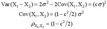
Consider point measurement deviations X1 and X2 taken at two points on a surface that are separated by a specified rate of change interval, denoted b. Assume that X1 and X2 are both N(0, s2). We wish to control the correlation of X1 and X2 so that the standard deviation of X1- X2 is some specified fraction of s, which we will denoted as c.

 

 

Since the correlation will be near one for a small spacing and near zero for a large spacing it is reasonable to model the correlation as a Gaussian function whose parameters are determined by the value of c. The function which expresses this correlation as a function of the sample spacing is called the autocorrelation function, and is denoted RX(t), where t is the distance between two samples. Hence RX(b) = rX1,X2.

 

The method of producing correlation between samples will be to apply independent normal distributions, N(0, s2), to each point, and then replace each point by a weighted average of the surrounding points. Resultant points that are close to each other will share the same heavily weighted original points and thus be highly correlated. Resultant points that are far apart will not share the same heavily weighted points, and thus will have a low correlation. The objective is to determine a weighting function, W(x), that produces the desired Gaussian autocorrelation function.

 

Open Surface Analysis

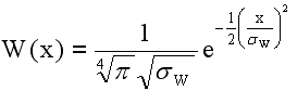
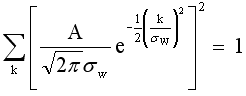
For purposes of simplicity, the weighting function will be assumed initially to be continuous over a line with infinite extent. The proposed weighting function is

 

 

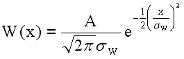
such that

 

 

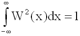
This condition is chosen so that each resultant point will have the same variance as the original point. Doing the integration yields

 

 

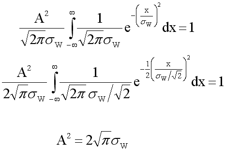
Now all we need is to determine sW in order to have W(x) completely specified.

The autocorrelation function for additive white Gaussian noise with a non-periodic function is

 

 

 

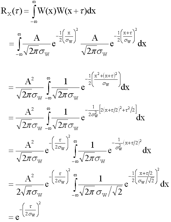
The autocorrelation produced by the proposed weighting function has the desired Gaussian form. If the reason behind the earlier choice of A2 was obscure, it should be clear at this point that this choice can also be justified as necessary so that RX(0) = 1.

Since b is the rate of change interval

 

 

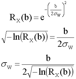
We now have W(x) completely specified as a function of the desired autocorrelation for a rate of change interval b.

 

 

Open Surface Implementation

Since lines do not have infinite extent and we only have discrete samples, W(x) will have to be modified slightly.

The first modification is that only a range of 12sW + 2b will be utilized in the discrete case, rounded up to span the next odd sample interval. We will retain the condition that the sum of the squared weights must be equal to one.

The finite line must be temporarily extended on each side by a number of points equal to (number of weights – 1) / 2 so that the W(x) will have the correct domain. In the language of digital filter theory these extra points compensate for the positive and negative lag of the filter.

W(x) can be applied using discrete Fourier techniques, and the extension of this analysis from a line to a surface is straightforward. The mesh of discrete points is processed as a rectangular, equally spaced grid that has been wrapped around the actual contour. The two directions need not have the same spacing.

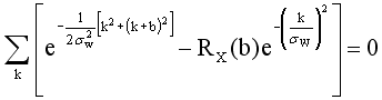
The second modification is that the value of sW must be altered slightly to set the discrete autocorrelation of two points separated by a sample interval b to exactly RX(b). The two pertinent equations are

 

 

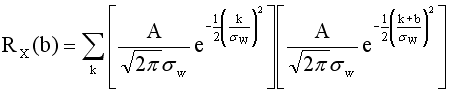
and

 

 

The second equation just sets the sum of the squares of the weights equal to one.

The factor A can be eliminated to yield a single equation in s that can be solved using the Newton-Raphson method, taking sW from the continuous case as the initial estimate for the discrete case.

 

 

It should be noted that b and sW are both in units of sample spaces, and k is the sample index.

 

Closed Surface Analysis

For a closed surface W(x) and RX(t) are both periodic. As with the open surface analysis we will initially assume that W(x) is continuous. The proposed weighting function is

 

 

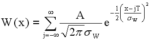
where T is the period of the closed surface.

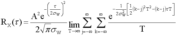
In the previous case we found that we did not have to derive the value of A up front. With that in mind, here we will start analyzing RX(t) first and find the value of A along the way. The autocorrelation function for additive white Gaussian noise with a periodic weighting function is

 

 

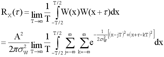
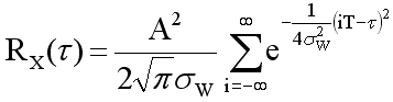
Completing the square on x and evaluating the integral leads to

 

 

If we let i = k - j, manipulate the limits, and complete the square on i we get

 

 

Since RX(0) = 1,

 

 

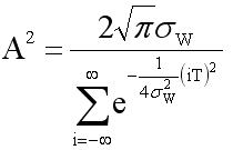
Which gives us

 

 

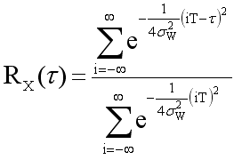
Since we know RX(b), we can solve for sW using the Newton-Raphson method. W(x) is now completely specified.

 

Closed Surface Implementation

As with the open surface case we only have discrete samples, so W(x) will have to be modified slightly, much as before. We will comment only on the main difference between the cases.

Since W(x) is periodic there is no lag for which to compensate. However, since the Fast Fourier Transform requires that the number of inputs is a power of 2, the number of mesh points on the closed surface must be a power of 2.

 

Conclusion

Some work remains to encompass this simulation technique within the larger scope of degree-of-freedom feature variation algorithms. This method may also suggest additional analysis and simulation strategies.

As it is, the Gaussian weighting function is a major improvement over current methods of simulating profile tolerances. It is controllable and can be justified from a process perspective.