Sequence Optimizer (SeqOpt) will use the JoinOpt_Tutorial model to find the optimal joining sequence for a set of joins. The Sequence Optimizer is used in compliant models to minimize assembly variation and/or process time.
•Launch 3DCS Variation Analyst. The AAO toolbar should be available.
•Open the JoinOpt_Tutorial model from
C:\Users\Public\Public Documents\DCS\3DCS_V5_8_2_0_0\Tutorials\V5SWMCNXV6CREO_AAO_Tutorial\JoinOpt_Tutorial
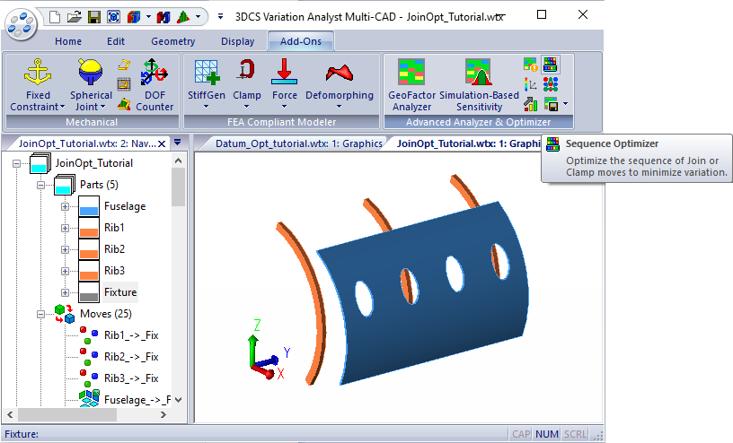
•This model includes:
- Five parts: 1 Fuselage, 3 Ribs, and 1 Fixture
- Rigid moves: Step Plane and Three Point
- Compliant moves: Load FEA, Clamps, Gravity, Joins, Unclamps
- Measures: Point Distance and Force
The model uses gravity to deform the Fuselage before the joins are applied. Sequence Optimizer will show that the final assembly is influenced by these joins, and by the order in which they are executed. The mesh files use solid mesh due to their thickness; this will result in large forces throughout the model.
After executing the rigid moves all distance measurements have a nominal value of 0.00mm and all nodal force measurements are 0.00N. Compliant moves will cause the parts to deform and the measurements in the model will show where the deformation will happen the most. Similarly, the nodal force measurements at the joining locations on Fuselage will show the tension introduced in the part. There will be 4 types of analyses to show improvement after optimization:
1. Minimization from Nominal
2. Minimization from Average
3. Minimization of Force
4. Minimization of Travel Path
STEP 1- Initial Results
| 1.1 | Nominal Build the model. |
| 1.2 | Run Analysis: 2000 samples. Name the simulation JoinOpt_Tutorial.hst |
| 1.3 | Save Simulation results as JoinOpt_Tutorial.csv |
STEP 2 - Minimization from Nominal - the optimized sequence will have the closest nominal values to the Design Nominal for distance and angle measurements.
| 2.1 | Nominal Build the model. |
| 2.2 | Go to the Advance Analyzer and Optimizer toolbar and select the |
2.2.1 Click the [Select Move (Join or Clamp)] button to add all 15 join moves in the model.
2.2.2 Select Minimization from Nominal for the Objective Function
2.2.3 Select All Measures from the Select Measure dialog ( the Select Measures... option under Measure will open the dialog)
2.2.4 Set Simulations number to 10
2.2.5 Select number of Threads to be used for the calculation. Type in a number equal to or less than the number of logical processors available on user's computer (that can be used during the calculation)
| 2.3 | Click the [Run Evaluations] button to start the optimization process. When completed the Optimization/Index column and the Optimal with the optimal Trial # will be populated. The Bar Chart is being populated with 105 blue and red bars, one set for each trial. The blue bar represents the Improvement from Baseline and the red bar represents the Travel Path (distance between two operations). This optimization focuses on blue bars only. |
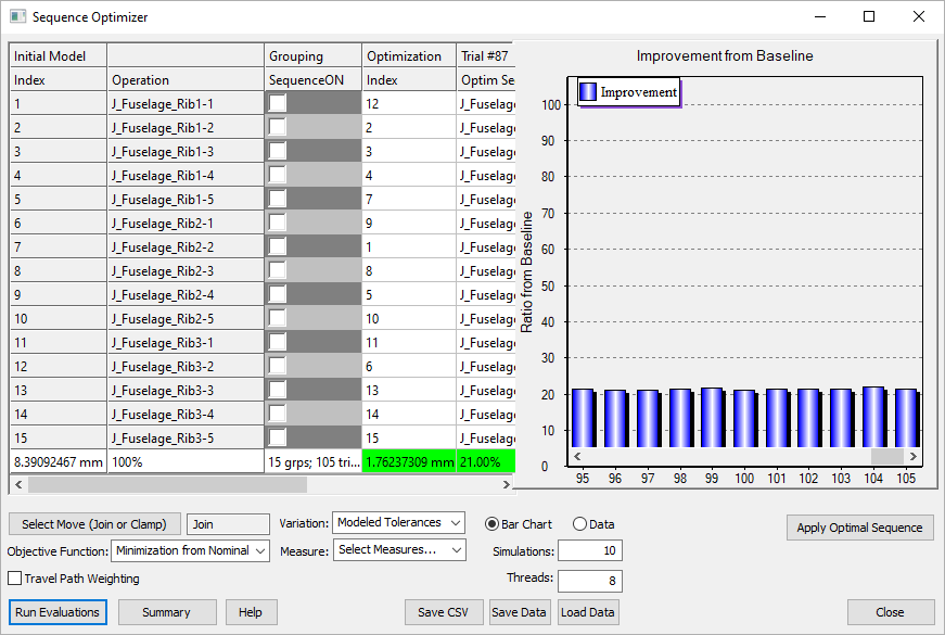
>>>Your results may not match the above illustration<<<
2.4 Interpreting the results: the new order of joins reduced the Initial value of 8.39 to the optimized value of 1.76 which represents 21.00% out of the initial 100%. Trial #87 shows the Optimal Sequence.
2.5 Use Save Data to save the Sequence Optimizer results. Name the file JoinOpt_Tutorial_dist.jop
2.6 Use the [Apply Optimal Sequence] to reorder the joins in the model as per the optimal sequence found during optimization. [Nominal Build] the model and run the analysis with 2000 samples. Name the simulation JoinOpt_Tutorial_dist.hst
2.7 Save Simulation results as JoinOpt_Tutorial_dist.csv.
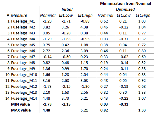
2.8 The results of the initial and optimized simulation runs are compared in the table below. The 14 measurements Nominal, Est.Low and Est.High values are compared. The nominal gaps are varying between -1.73mm and 4.48mm for the initial joining order. That range of values is reduced in the optimized sequence to numbers between 0.03mm and 0.82mm, a much smaller range. These new set of Nominal values are also improving the Curve Fit values for Est.Low and Est.High. The optimized results are reducing the nominal gaps, thus reducing the deformation of the part.
2.9 In the Bar Chart area scroll all the way to the left and left-click on the first blue bar. This will replace the Optim Seq with Select Seq and the Trial #87 will become Trial #0 (the original order of joins). Then right-click on the same blue bar and select the Apply Sequence option: this will reorder the joins in the model to match the original sequence.
STEP 3 - Minimization from Average - the optimized sequence will have the smallest variation from Mean values for distance and angle measurements.
| 3.1 | [Nominal Build] the model. |
3.2 In the Sequence Optimizer dialog set these inputs:
3.2.1 Click the Select Move (Join or Clamp) button to add all 15 join moves in the model.
3.2.2 Select Minimization from Average for the Objective Function
3.2.3 Select All Measures from the Select Measure dialog.
3.2.4 Set Simulations number to 10
| 3.3 | Click the [Run Evaluations] button to start the optimization process. When completed the Sequence Optimizer dialog looks as shown here: |
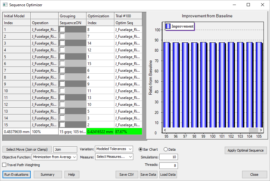
>>>Your results may not match the above illustration<<<
3.4 Interpreting the results: the new order of joins reduced the Initial value of 0.48 to the optimized value of 0.42 which represents 87.67% out of the initial 100%.
3.5 Use [Save Data] to save the Sequence Optimizer results. Name the file JoinOpt_Tutorial_avg.jop
3.6 Use the [Apply Optimal Sequence] to reorder the joins in the model as per the optimal sequence found during optimization. [Nominal Build] the model and run the analysis with 2000 samples. Name the simulation JoinOpt_Tutorial_avg.hst
3.7 Save Simulation results as JoinOpt_Tutorial_avg.csv
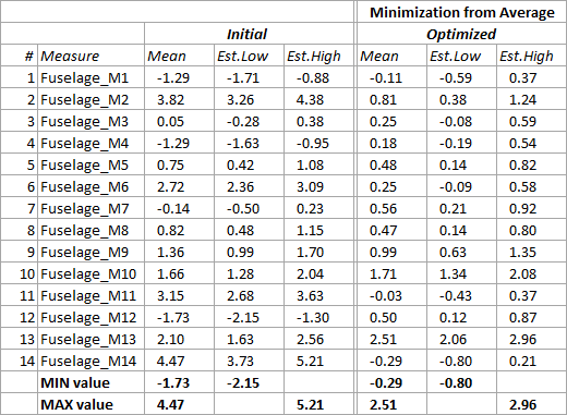
3.8 The results of the initial and optimized simulation runs are compared in the table below. The 14 measurements Mean, Est.Low and Est.High values are compared. The Mean value is varying between -1.73mm and 4.47mm for the initial joining order. That range of values is reduced in the optimized sequence to numbers between -0.29mm and 2.51mm, a much smaller range. These new set of Mean values are also improving the Curve Fit values for Est.Low and Est.High and also reducing the deformation of the part.
3.8 In the Bar Chart area scroll all the way to the left and left-click on the first blue bar. This will replace the Optim Seq with Select Seq and the Trial #100 will become Trial #0 (the original order of joins). Then right-click on the same blue bar and select the Apply Sequence option: this will reorder the joins in the model to match the original sequence.
STEP 4 - Minimization of Force - the optimized sequence will have the smallest values for force measurements.
| 4.1 | [Nominal Build] the model. |
4.2 In the Sequence Optimizer dialog set these inputs:
4.2.1 Click the [Select Move (Join or Clamp)] button to add all 15 join moves in the model.
4.2.2 Select Minimization of Force for the Objective Function
4.2.3 Select All Measures from the Select Measure dialog. Force optimization will bring up a different set of measurements: the nodal force measurements instead of the distance measurements.
| 4.3 | Click the [Run Evaluations] button to start the optimization process. When completed the Sequence Optimizer dialog looks as shown here: |
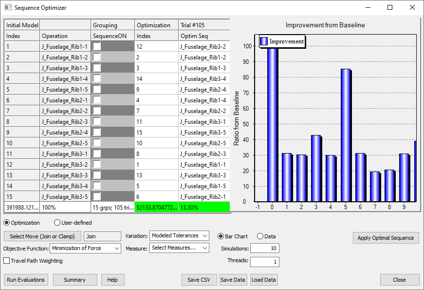
>>>Your results may not match the above illustration<<<
4.4 Interpreting the results: the new order of joins reduced the Initial value of 391988.12N to the optimized value of 52133.87N which represents 13.30% out of the initial 100%.
4.5 Use [Save Data] to save the Sequence Optimizer results. Name the file JoinOpt_Tutorial_force.jop
4.6 Use the [Apply Optimal Sequence] to reorder the joins in the model as per the optimal sequence found during optimization. [Nominal Build] the model and run the analysis with 2000 samples. Name the simulation JoinOpt_Tutorial_force.hst
4.7 Save Simulation results as JoinOpt_Tutorial_force.csv
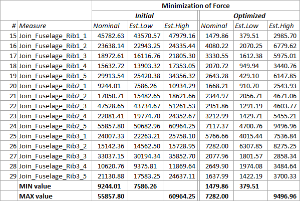
4.8 The results of the initial and optimized simulation runs are compared in the table below. The 15 measurement's Nominal, Est.Low and Est.High values are compared. The Nominal value is varying between 9244.01N and 55857.80N for the initial joining order. That range of values is reduced in the optimized sequence to numbers between 1479.86N and 7280.00N, a much smaller range. These new set of Nominal values are also improving the Curve Fit values for Est.Low and Est.High and also reducing the stress in the part.
4.9 In the Bar Chart area scroll all the way to the left and left-click on the first blue bar. This will replace the Optim Seq with Select Seq and the Trial #105 will become Trial #0 (the original order of joins). Then right-click on the same blue bar and select the Apply Sequence option: this will reorder the joins in the model to match the original sequence.
STEP 5 - Minimization of Travel Path - the optimized sequence will have the shortest 'travel distance' between all operations. The 'travel distance' is the sum of all distances (3D true distance) measured between two consecutive operations. This calculation should be used in conjunction with one of the first three calculations. The Travel Path Weighting can be used to balance the importance of Travel Path vs Minimization calculations.
In this example we'll Minimize the Travel Path while also Minimizing from Nominal.
For this model the joins are already in the best order for the Travel Path optimization. Therefore, any optimization that includes Travel Path will result in a longer path than the original one.
5.1 Open the Sequence Optimizer and load the JoinOpt_Tutorial_dist.jop file. Apply Optimal Sequence to the model; now the joins are in the best order to minimize the nominal values for all distance measures. Close the Sequence Optimizer.
5.2 Reopen the Sequence Optimizer dialog and set these inputs:
5.2.1 Click the [Select Move (Join or Clamp)] button to add all 15 join moves in the model.
5.2.2 Select Minimization from Nominal for the Objective Function
5.2.3 Select All Measures from the Select Measure dialog.
5.2.4 Set Simulations number to 10
5.2.5 Activate the Travel Path Weighting and leave the Weighting Factor at 0.5. This will give the Travel Path same chances to be optimized as the Minimization from Nominal (this last optimization is going to be further improved if possible).
| 5.3 | Click the [Run Evaluations] button to start the optimization process. When completed the Sequence Optimizer dialog looks as shown here: |
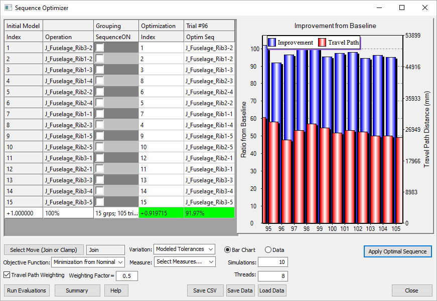
>>>Your results may not match the above illustration<<<
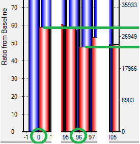
5.4 Interpreting the results: Since both Minimization from Nominal and Travel Path are optimized the results show a reduced value of 91.9% out of the initial 100% for both, the Minimization from Nominal and the Travel Path.
You can observe the Travel Path reduction in the image below where Trial #0 and Trial # 96 are shown side by side:
5.5 Use [Save Data] to save the Sequence Optimizer results. Name the file JoinOpt_Tutorial_dist_TP.jop
5.6 Use the [Apply Optimal Sequence] to reorder the joins in the model as per the optimal sequence found during optimization. Nominal build the model and run the analysis with 2000 samples. Name the simulation JoinOpt_Tutorial_dist_TP.hst
5.7 Save Simulation results as JoinOpt_Tutorial_dist_TP.csv
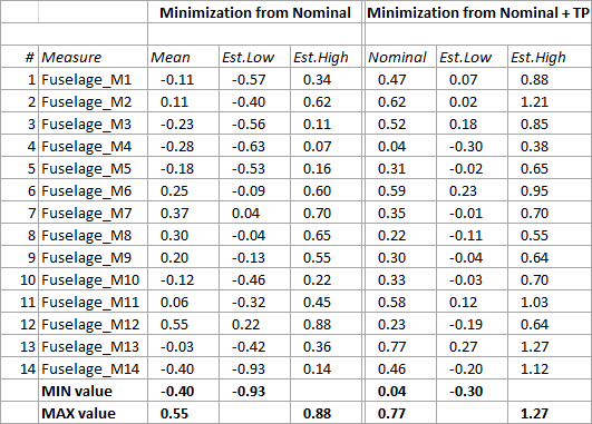
5.8 The results of the initial and optimized simulation runs are compared in the table below. Overall the Nominal values seem to be slightly closest to each other, with a slight mean shift.