SBS provides insight into the interactions between multiple inputs, and how those interactions may affect an output's mean. What-If experiments gain a high level of accuracy and speed because of SBS analysis. SBS runs hundreds or thousands of samples and compares the tolerance range to the measure range.
Characteristics of SBS: ▪Results are based on full simulation runs ▪Better predictability ▪Deeper understanding of the model ▪Contributions for interactions between tolerances ▪Contributions to mean shift
Applications for SBS: ▪Measures with one-sided spec limits ▪Conditional logic ▪Tolerances that interact (e.g. Positional tolerances with Bonus) ▪Unilateral tolerances ▪Constant Offset tolerances
|
SBS is part of the Add-On menu named Advanced Analyzer and Optimizer.
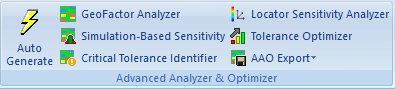
Double-click the Simulation-Based Sensitivity button to launch the DOE Regression Table.
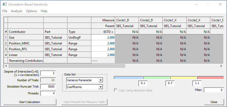
This dialog lists the input tolerances with their ranges and the part they belong to, one on each row. The measurements at the top. No calculation is performed at this point.
User input
1. Degree of Interaction[1-6] - Represents the number of contributors that will be considered concurrently and calculate the effect their interaction will have on each measure. Default number is 2, meaning that the effect of each two tolerances at the time will be considered. The interaction for a pair of tolerances is calculated by adding the results with both "on" and all other tolerances "off" and subtracting both sets of the results with just one of the two tolerances "on". Higher degrees of interaction are calculated with similar but longer equations. They are isolating the effect of the set of tolerances from the effects of the subsets of tolerances.
Note: Bonus tolerance is calculated as a combination of size and position tolerance so it will only appear as one of the interaction contributors.
2. Simulation Runs per Trial - Is the number of simulations (assemblies) to be built (same as the regular Simulation)
Based on the Degree of Interaction selected a Number of Trials will be set. The trial number = contributor number + 1, where 1 is for the base calculation (i.e. Deviate to Offset calculation). Most tolerances do not have an offset so the first run will do nothing but if some of the tolerances are not equal-bilateral then the first run is used for that propose, apply the offset value to tolerances.
In the picture above the Number of Trials is 11, meaning that for each one of the 5000 simulation runs there will be 11 combinations of input tolerances. If the Degree of Interactions is changed to 1 the Number of Trials becomes 5, based on the 4 input tolerances.
3. Threads - Is the number of computer cores used during calculation. At the moment up to eight cores can be used simultaneously. There will be some difference in the Simulation results between runs with Thread = 0 and runs with Thread = 1, 2, 3,...,8 because for the former the seed selection is random while for the latter the seeds are selected prior to running the analysis.
Data Set (drop-down lists)
First set of options are:
•Variance Parameter - The sigma-based values will be displayed (the square roots of the values in the equations).
•Mean Parameter - The mean shift values will be displayed.
Second set of options are:
•Coefficients - Represent the ratio between the tolerance or float range (or offset) and the measure 'n'-STD or mean shift and they are similar to the G Factor values generated in Geo Factor and AAO. Basically, a high coefficient only means the user may need to change something - maybe the design, maybe the assembly process, etc. The Coefficients will be the same as G Factor values only in a linear model, without interactions between the contributors and all normal distributions. Otherwise, the results will be different because the terms represent similar but not identical values.
To calculate the Coefficient of a particular contributor, SBS runs a simulation with the range of that contributor set to 'x' and all other ranges set to 0.000001 (not zero to preserve the random number stream.) The measure 'n'-STD for a particular measure will be an Amount 'y'. Therefore, the Coefficient for the contributor-measure pair will be y/x. Since neither the contributor range nor the measure 6STD can be negative, the coefficients for the direct contributors will always be positive (there are some exceptions.)
•Percentages - The percent contributions in SBS are calculated directly from the Amounts, so they directly reflect the simulation results.
•Amounts - The 'n'-STD value for each measurement calculated for each contributor. Because the Amount for a particular interaction of contributors involves subtracting measure results, it can and will often be negative. A negative Amount means the combined effect of the contributors decreases or mitigates the expected measure 'n'-STD result as compared to an RSS stack. An interaction with a negative Amount will also have a negative Percent Contribution.
Everything SBS does to predict the measure 'n'-STD (Variance) it also does to predict the measure Mean results too. SBS uses the same terms (Amounts and Coefficients) for the Mean analysis, where negative values (Amounts and Percent Contribution) indicate the mean shift is getting smaller or more negative. Positive values indicate the mean is increasing.
Action buttons
1. Start Calculation will start the simulation run and calculate the contributors based on all simulation builds. A Running Simulation-Based Sensitivity dialog will appear showing the calculation progress. When finished the Simulation-Based Sensitivity dialog is updated as show below.
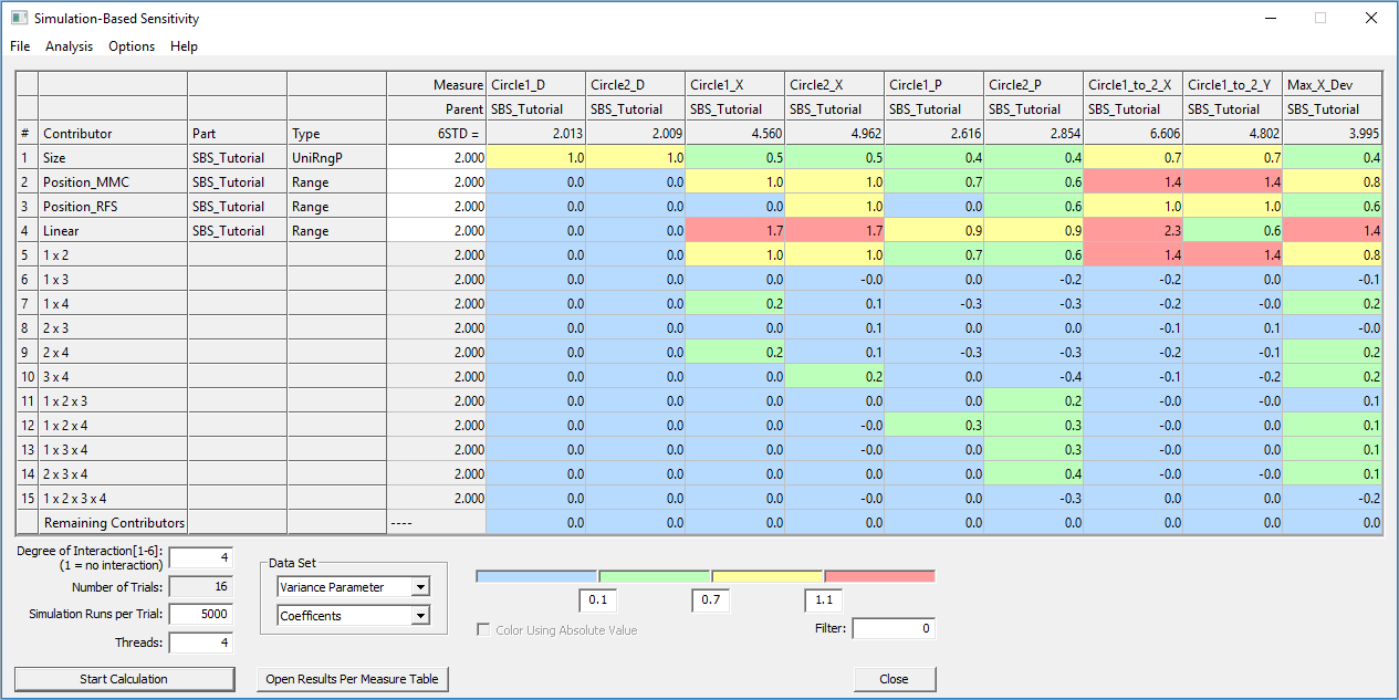
![]() Notice that the number of rows in the above table is now 15 instead of the initial 4 because the input for Degree of Interaction was set to 4. This results in an additional row for each combination of the initial 12 contributors,up to four at the time.
Notice that the number of rows in the above table is now 15 instead of the initial 4 because the input for Degree of Interaction was set to 4. This results in an additional row for each combination of the initial 12 contributors,up to four at the time.
The calculation will first find the Amount value (from the simulation runs) and then the Coefficient. This process may take a long time, depending on the size of the model, number of contributors and number of Degrees of Interactions selected by the user.
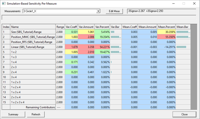
2. Open Results Per Measure Table - Will open a new table that displays the Coefficients, Amounts and Percentages for both Variance and Mean for each measurement. Each measurements can be viewed by selecting it in the Measurements drop-down list. The Edit Meas button opens the displayed measure dialog for editing.
Menus
File menu
1. Load SBS File - Will load a previously saved SBS file.
2. Save SBS File - Will save a *.sbs file that can be later loaded back into the Simulation-Based Sensitivity dialog. Sometimes running the SBS calculation can take a long time, therefore the *.sbs file helps avoiding re-running the analysis and also with comparing results for different settings.
3. Export to CSV - Will save the DOE regression results to a csv file.
Analysis menu
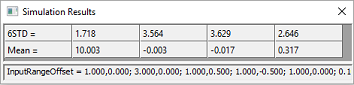
1. Run Simulation - Will run the Monte Carlo simulation for the same number of samples as the one used in the Simulation-Based Sensitivity dialog. The results displayed are the 'n'STD and Mean for all measurements. The range and offset values for input tolerances are also displayed.
2. Refresh from Model - will update the information in the Simulation-Based Sensitivity dialog to match the model tolerances and measures.
3. Restore Ranges - Once the SBS table is generated, the user can change the contributor ranges and predict the new measure results, assuming the Coefficients represent linear contributor/interaction and measure relationships. It is still recommended to confirm the new results with a simulation run. The Restore Ranges button will replace whatever ranges the user modified with the original ones from the model.
4. Apply ranges to tolerances - will update the model tolerances range and offset value to match the values displayed in the Simulation-Based Sensitivity dialog.
5. Apply ranges at selected trial to tolerances - For each Trial all tolerances except the selected one are set to 0.000001. E.g. for Trial = 4 ( in the image above) all tolerances except Linear(SBS_Tutorial).Range will be set to 0.000001. Applying this command will set the tolerances in the model to the values assigned to the selected Trial (row) in the Simulation-Based Sensitivity dialog.
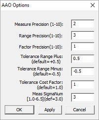
Options menu - Allows setting the default values for measure, tolerance and factor (coefficient) decimals.
|
•Measure Precision: Changes the decimal place value for Measures, across the top of the GeoFactor Analyzer, SBS and CTI dialogs. •Range Precision: Changes the decimal place value for the Tolerance Range value for GeoFactor Analyzer, Simulation Based Sensitvity (SBS), Critical Tolerance Identifier (CTI), Tolerance Optimizer, LSA dialogs. •Factor Precision: Changes the decimal place value of the Factors or overall display of the GeoFactor Analyzer dialog. •Tolerance Range (Plus/Minus): Applies to the Critical Tolerance Identifier (CTI) dialog, changing the affective tolerance range for the Target 6-Sigma. •Tolerance Cost Factor: Changes the Cost Factor value in the Critical Tolerance Identifier dialog. •Measure Sigma Num: Changes the Sigma value for Measures in GeoFactor Analyzer, Simulation Based Sensitivity, |
RH Menus
Use the right-hand mouse button anywhere in the DOE Regression Table to bring up the following commands:
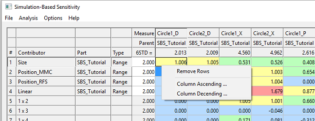
1. Remove Rows - Use Ctrl or Shift keys to select multiple rows then right-click and select Remove Rows. The selected rows are removed from the list. Their contribution will be displayed as a combination in the "Remaining Contributors" row (the last row).
2. Column Ascending - Will reorder the rows in ascending order based on the selected column.
3. Column Descending - Will reorder the rows in descending order based on the selected column.
Other settings
1. Filter: When the rows have all numbers smaller that the Filter value, they will be hidden.
2. Legend: Allows setting values that will color the coefficients based on these values for a better visual identification of critical coefficients/tolerances.