Through the measure's dialog we could see the variation on a build-by-build basis, but we were not getting any statistics that we could later use to make a design decision. To really get a complete look at our population of samples and understand the potential risk of our design, we need to move to the Simulation analysis. The Simulation analysis within 3DCS will analyze the measured variation for the assembly. It works by using a Monte Carlo random number generator to randomly add variation according to the individual tolerancing information specified. Then it will assemble the deviated parts and take the measurements. The Simulation will compile the results from these measurements for each simulated assembly. The results of the Simulation will be displayed as a histogram in a separate window.
The Contributor Analysis is another useful analysis tool within 3DCS. This will determine the sources of variation for a particular measure and rank them according to their percentage of contribution.
•Click ![]() Nominal Build.
Nominal Build.
•Click the ![]() Run Analysis button to bring up the Run Analysis dialog.
Run Analysis button to bring up the Run Analysis dialog.
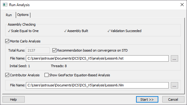
•The Total Runs will default to 2137 with Recommendation based on convergence on STD enabled. In the Options tab it is possible to adjust inputs and have 3DCS recommend how many runs to do until convergence to a certain confidence. For this analysis, leave it as the defaults.
•Ensure that Monte Carlo Analysis and Contributor Analysis are both checked on and Show GeoFactor Analysis is unchecked.
The Initial Seed is the starting point for the random number generator. Keep this number the same when you are trying to produce identical results from two simulations. Next to Initial Seed in the Run Analysis dialog there is the number of Threads which allows users to utilize multi-core processing to run an analysis faster at the cost of more computing power. The maximum Threads allowed with one 3DCS license is 8. This is a simple analysis so regardless of how many Threads we use it will run quickly so this input is not important. Initial Seed and Threads can be changed in the Options tab.
•Click the [Start>>] button.
•If you see warnings that the *.hst and *.hlm files will be overwritten, click [Yes] to ignore the warnings.
You will be shown a counter to display the Simulation progress. After all of the runs have been simulated, the Contributor Analysis will start automatically. After both analyses are completed, the Analysis Summary window will open to display the results.
>>>Your results may not match the above illustration<<<
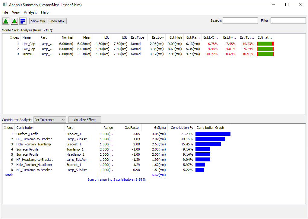
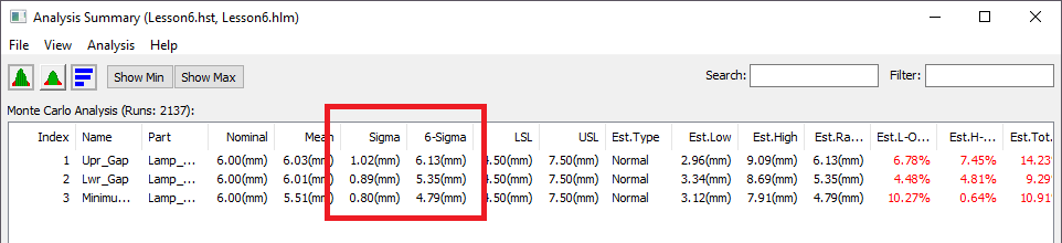
The Analysis Summary window shows us "at a glance" results for all of the measures in the model. The top half of the Analysis Summary window has information about the Monte Carlo simulations (the 2000 runs) for all of the measures. The lower half of the Analysis Summary window shows information about the Contributor Analysis that 3DCS ran after completing the Monte Carlo simulations. The Contributor Analysis results are different for each of the measures, as tolerances will affect all measures differently. The Est. Range column in the top half of the window tells us an estimate (based on a curve-fit to a distribution of the data) of the amount of variation at each measure. Based on the Est. Range numbers, it appears that in our design we are seeing the most variation in the Upr_Gap measure.
•Double-click on Upr_Gap in the upper half of the Analysis Summary window to open the Analysis Results window for the Upr_Gap measure.
>>>Your results may not match the above illustration<<<
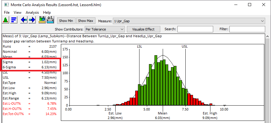
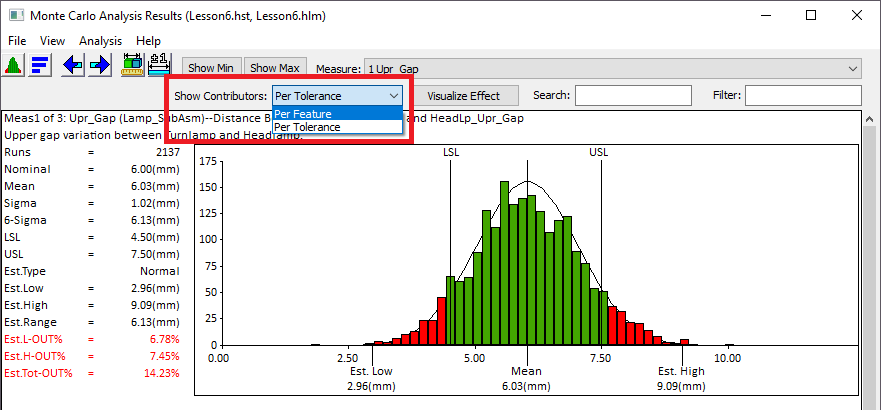
The top half of the Analysis Results window contains all of the information from the Monte Carlo simulations and the bottom half of the Analysis window contains the Contributor results. The most common value referenced when evaluating the range of variation is the 6-sigma value. Sigma is a Greek letter which is mathematically used to denote the Standard Deviation of a distribution. In the Analysis window, Standard Deviation is abbreviated as Sigma. Therefore the 6-Sigma value is the ±3 standard deviation range of variation for the particular measurement. If the 6-Sigma value isn't displayed on the upper left part of the screen with all of the other statistics, it can be turned on from the Analysis Options dialog as shown in the steps below.
•From the Analysis Results window go to View ![]() Options. This will bring up the Analysis Options dialog.
Options. This will bring up the Analysis Options dialog.
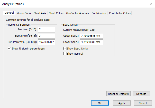
From the Analysis Options dialog several settings in the Analysis Results window can be changed such as number of decimal places, displayed statistics, or contributor fields to name a few. However, in this tutorial we will simply add the 6-sigma field to the statistics.
•Navigate to the Monte Carlo tab and in the Statistics to Display section turn on the Sigma and 6-Sigma statistics.
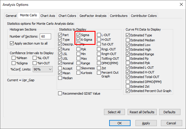
•Select [OK] to save and close the Analysis Options dialog. Notice that two fields have been added to the field in the Analysis Results window and two columns have been added to the top half of the Analysis Summary window. This will happen for any statistics you choose to add to your results display in your model.
Standard Deviation is most meaningful if the data is normally distributed. The Estimated (Est.) Range is the difference between the Estimated High and Estimated Low values. These values are derived from a curve fit to the samples. If the data is normally distributed, the Est. Range will match the 6-Sigma.
In addition to the Simulation results, the Analysis Results window also contains the Contributor Analysis results. The Contributor Analysis results are displayed below the Simulation results. 3DCS calculates what percentage of the variation is coming from each contributor. Because the Contributor Analysis is run independently of the Monte Carlo simulations, it is not guaranteed that the variation will decrease by exactly the percentage that the Contributor Analysis is predicting but it is typically pretty close. The Contributor Analysis can be presented in two different ways, either Per Tolerance or Per Feature. Because 3DCS allows users to put all features associated to one callout within one GD&T dialog, it can then sum up the contributions of all those features and give an overall contribution number for that callout. These are the results that are shown for Per Tolerance. If instead of seeing the results summed up you'd rather see the results for individual features, 3DCS offers that information too in the Per Feature results.
•In the Analysis Results window toggle to Per Feature in the Show Contributors drop-down shown below.
With Per Feature selected the Contributor Analysis results will look similar to those displayed below.
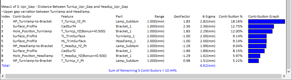
One critical value that requires more explanation is the GeoFactor value. The GeoFactor value is meant to communicate the magnifying or mitigating effect that the design geometry has for that tolerance. For example, a GeoFactor of 2.00 would mean that 1mm of change at that tolerance location will yield 2mm of change at the measured location. Something in the geometry is allowing that tolerance to have a large effect on our measured variation.
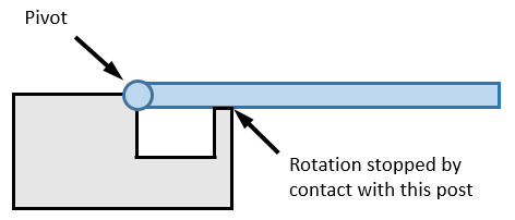
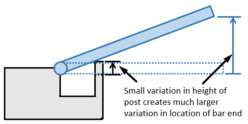
In the example above, a small change in the height of the post has led to a very large change in the location of the end so the tolerance controlling the height of the post will have a GeoFactor value much greater than 1 for a measure checking the location of the end in the direction shown.
In this model we have three measures but we primarily only focused on one in this lesson. Each measure will have a page of Simulation and Contributor Analysis results.
•Close the Analysis windows when you are finished looking at the results.
•Click ![]() Separate.
Separate.