The
|
Input:
Distribution: Required
Magnitude
All parameters required
Name
Required
Direction
Required
Point List
Required
Angular Options
Required
Description
Optional
Methodology:
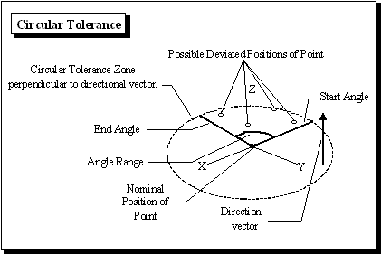
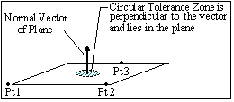
The tolerance varies in a circular tolerance zone which is perpendicular to the specified direction vector.
STEP 1
The magnitude by which the point has to be deviated in a circular zone, is calculated from range, offset, ( or plus & minus), distribution, sigma, truncation, and scale values. This determines the distance that the point will be deviated from the nominal center.
STEP 2
The point is deviated by the magnitude and then is rotated from the start angle to a random angle. The random angle is determined by the angular range (plus & minus), distribution, sigma, truncation, and scale values. The angle is measured in the plane, perpendicular to the direction vector.
How is Bonus Tolerance handled?
When a circular tolerance is applied to the center of a circular feature (circle, hole, pin, cylinder ) and the feature is at MMC (Maximum Material Condition) a "Bonus Tolerance" is added to the circular tolerance.
Maximum Material Condition, or MMC, is the condition where the most amount of material is present.
•A hole is at MMC when it is at its smallest size. Similarly a pin is at MMC when it is at its largest size.
•As the circular feature departs from MMC, bonus tolerance is added to the circular tolerance range. If the tolerance is set to Group mode, the smallest size deviation of all the features is used to calculate the bonus tolerance. If the tolerance is set to Composite mode, the bonus tolerance is calculated separately for each feature and applied to the the independent range (Rand#3).
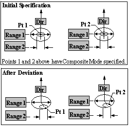
Parameters - Mode, direction vector, angular definition and multiple scale which defines the angular variation of a circular tolerance, have been outlined below as specific parameters.
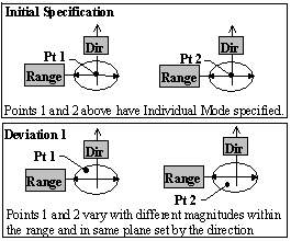
Mode selection: Specify the mode option for the tolerance. The mode field lets you specify different combinations of magnitude and direction, for greater flexibility. The mode option has three choices: Individual Mode, Group Mode and Composite Mode.
Individual Mode: When Individual Mode is specified, each point in the list that is associated with the tolerance varies:
•With different magnitudes and angles in the specified ranges.
•In the plane of the one specified direction vector.
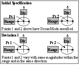
Group Mode: When Group Mode is specified, each point in the list that is associated with the tolerance varies:
•With the same magnitude and angle in the specified ranges.
•In the plane of the one specified direction vector.
•Always verify the points' Associated directions when using Group Mode. .
Composite Mode:
•The range values are the same as the tolerance values from the feature control frame.
•RightSkew distributions are required (except for worst case analysis.)
•No Offset should be applied to either Rand. Index.
•Always verify the points' Associated directions when using Composite Mode.
•The ranges for Rand#1 and Rand#3 are RSSed (unless the distributions are set to Modal, BiMode, Step, Constant, or UserDef. For these distributions, the ranges are subtracted to support worst case analysis.)
Direction: Specify the Vector direction for the tolerance.
•Type In Method
•Two Point Method
•Normal Direction Method
•AssocDir Method
•PickPtDir Method
Type In Method: Varies a point in the direction of the vector that is normal to the selected plane. Select 3 points to specify the plane along whose vector the tolerance is applied.
Two Pt Direction Method: Varies a point in a direction normal to the vector of the line segment chosen. Select a line segment (2 points) normal to which the circular tolerance is applied.

Normal Direction Method: Specify the vector along which direction the tolerance is applied.

The purpose of this section is to explain the use of the Rayleigh distribution in the 3DCS circular tolerance. The Rayleigh distribution is a specific case of the Weibull distribution, and at present the software only uses the more general Weibull name.
There are two questions that must be kept firmly in mind to understand why the Rayleigh distribution is used as the circular tolerance magnitude.
1. What is being simulated?
2. How is the simulation performed?
What is being simulated?
The goal is to simulate the error in a process that locates a feature relative to a target point. A familiar example of this is throwing darts. When playing darts the thrower aims in two directions, left/right and up/down, or x and y. This is representative of most manufacturing processes as well. Since this is the process that we are simulating, our default assumption is that the location of the holes on the dart board will be normally distributed in x and y.
How is the simulation performed?
The simplest way to simulate variation that is normally distributed in two directions is to apply one normal distribution in each direction. However, there is more than one way to get the desired result. Since circular tolerance is defined in terms of the magnitude of the deviation from a nominal location, dimensional management software has historically simulated circular tolerances using magnitude and angle distributions.
It is critical to keep in mind that the goal is to simulate variation that is normally distributed in x and y, even though the simulation is defined in terms of magnitude and angle distributions. Think back to throwing darts. The distribution of the holes in the dart board can be analyzed in terms of their magnitudes and angles, but the thrower still aims in x and y.
The question of how to perform the simulation is one of figuring out what magnitude distribution produces variation that is normally distributed in x and y when combined with an angle that is uniformly distributed, just as when throwing darts.
The first thing to do in understanding the use of the Rayleigh magnitude distribution is to perform two experiments in 3-Dcs. You should do this for yourself.
1. Apply two identical independent normal tolerances to a point in two directions and measure the pure distance of the deviated points from nominal. The histogram for the measurement has the Rayleigh distribution.
2. Apply a circular tolerance to a point with a Rayleigh (Weibull) magnitude and measure the deviations of the point in x and y. The histogram for each measurement has a normal distribution.
If you look at the scatter plots for the two experiments you will see that they have the same pattern, like the one shown on the next page. This should be enough to convince you that a Rayleigh magnitude distribution corresponds to normal distributions in x and y, even if it is not clear just why this is so.
Explanation
With a little calculus it can be proven on a purely theoretical basis that a Rayleigh magnitude distribution produces variation that is normally distributed in x and y. Instead of doing the calculus, let's do an experiment to demonstrate the point.
First, apply two identical independent normal tolerances to a point in two directions as before, and look at the scatter plot of 1000 points with rings imposed on it.
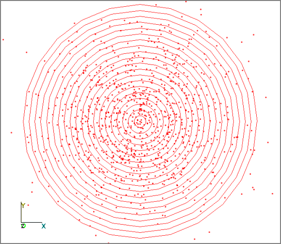
Now we will create the histogram of the magnitude measurement. We will do this in two steps by first moving each point of the scatter plot radially to the center of its ring. This will help make the critical observations clearer.
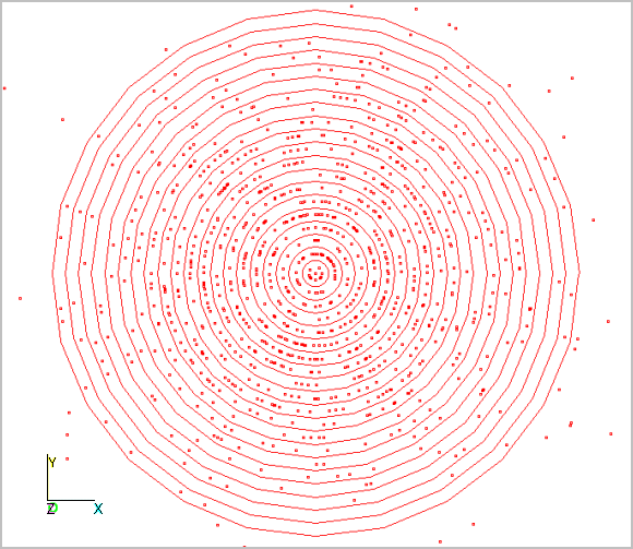
You should have been able to see that the density of points was highest at the center of the original scatter plot. However, the area of the rings increases away from the center, so the inner rings actually contain more points than the center circle. The number of points in each ring starts small at the center, increases to a peak around the eighth ring, and then tapers off in the outer rings. This gives us a good feel for what the histogram of the magnitude will look like.
Now we will actually make the histogram, with each ring of the scatter plot becoming a bar of the histogram. To get a nice histogram we will use 100,000 simulations rather than just the 1000 that were used in the scatter plots. The histogram is on the next page.
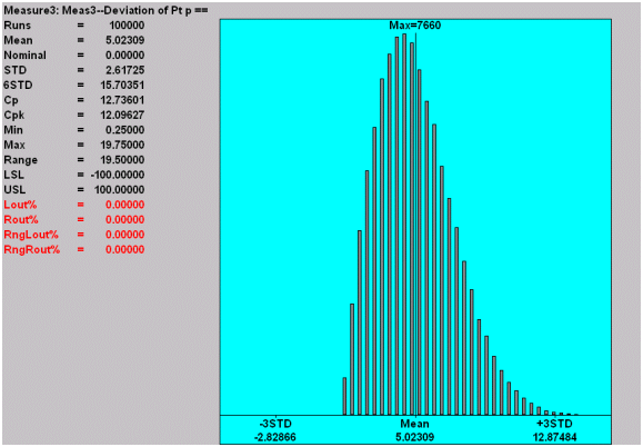
The pattern of the bar heights is just what we expected based on the observations from the previous scatter plot. This is a histogram of the Rayleigh distribution.
Another way to think about this relationship is to think of the points in each bar of the Rayleigh histogram as being evenly dispersed around a ring of a dart board. As the bars get further from zero the rings become larger, so the points in the upper bars are dispersed over a greater area, and the normal distributions in x and y are recreated.
This relationship between the Rayleigh magnitude and the Normal distributions in x and y is often not obvious at first glance, but this analysis should make it easier to understand.
Notes:If multiple tolerances are on the same feature (i.e.: Composite), you cannot have the same Truncation value for each frame in RSS mode. The Truncation is independent for each frame, so the total variation could exceed the location truncation.
|