The distribution types are used to show the type of variation. The following are the different types of distribution available.
See Also:DE Focus Article - Issue 25: Normal, Uniform, Triangle, Rightskew, Leftskew, OpenUp, OpenDown DE Focus Article - Issue 26: BiMode, Constant, Step, Weibull4, Modal, Pearson4 DE Focus Article - Issue 27: User-Defined;
|
|||
|
|
|
|
|
|
|
|
|
|
|
|
|
|
|
|
|||
2D Distributions: GD&T with diametrical zone, Circular Tolerances, and Move Floats. These distributions will be available by default. Users can hold the HOME key to select the 1D (legacy) Distributions. Uniform (Hockey Puck), Normal (Sand pile), Triangular (Cone) and Trapezoidal distributions similar to existing 2D Normal (Sand Pile) are supported in all GD&T with a diametrical zone, the Circular tolerances, and moves floats. |
|||
|
|
|
|
|


Normal: Gives the tolerance a normal distribution. This distribution is used for tolerances that are distributed according to a standard bell-shaped curve.
Normal-2D: Is applied as Bi-variate Normal, resulting in samples normally distributed at any section through the center.
Uniform: Every tolerance value in the defined tolerance range has the same probability of occurrence.
Uniform-2D: Any point in the circular zone is equally likely resulting in a Hockey Puck shape, with the samples uniformly distributed at any angle through the center.
Triangular: The curve reflects the shape of a triangle with a peak in the center.
Triangular-2D: The resultant shape for the samples is a Cone; Triangular at any angle through the center.
BiMode: Every tolerance value in the defined tolerance range has the same probability of occurrence only with the minimum and maximum values.
Right Skew: A normal shaped curve pushed to the right side indicating a higher probability of positive variation. (Ref: DE Focus Issue 25; Weibull Right)
Left Skew: A normal shaped curve pushed to the left side indicating a higher probability of negative variation. (Ref: DE Focus Issue 25; Weibull Left)
Open Up: A curve that looks like a convex surface, indicating a higher probability of variation at its extreme limits with very little variation in the center.
Open Down: A curve that looks like a concave surface, indicating a higher probability of variation at its center with very little variation at its extreme limits.
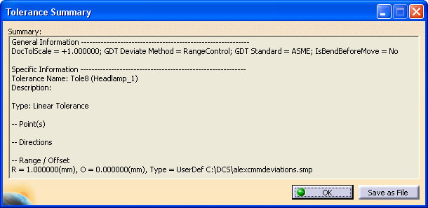
User Defined:A text file containing deviated values can be linked to a tolerance. The file should have extension SMP and be selected when this distribution is selected. See Capability Tolerance for a more comprehensive method to include measured data.
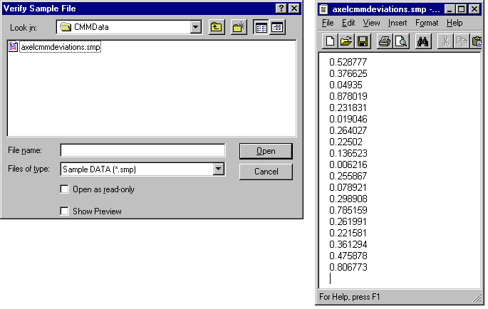
•The file path to the *.smp file in displayed the Summary.
Step Distribution: Every tolerance value in the defined tolerance range increments in steps of variation similar to a uniform curve. The distribution is specified by range (min/max) and segment number (segNum). The segment number is calculated based on the STEP Level (STEP Level - 1). By definition, this distribution is NOT a probabilistic distribution but it is very useful in simulating mean shift related variation (e.g., tool wear).
Constant: This distribution assigns the same value to the tolerance every time the tolerance is used. It is used in simulating float to the maximum allowed clearance.
•To validate the results of the Float, deactivate all other tolerances, leaving only one float active, and run a new Simulation.
•Review the 6-Sigma of the Contributor Analysis, the GeoFactor Estimated Range and the 6-Sigma results in the Monte Carlo Simulation results should match.
•In a move, the Float uses the LMC size. (Smallest Pin, Largest Hole).
Switching from Constant distribution to another distribution, will reset the Offset field value to. (70621) |
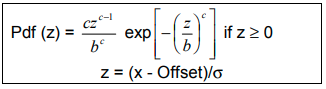
Weibul4: This is a generic distribution, controlled by four parameters: Offset, Sigma (σ), Scale (b), and Shape (c). The Offset and Sigma parameters are set on the Edit Feature Tolerance dialog
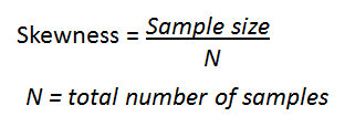
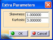
Pearson4: This is a generic distribution, controlled by four parameters: Offset, Sigma, Skewness, Kurtosis. The Offset and Sigma parameters are set on the Edit Feature Tolerance window.
Note: Clicking on the Pearson4 button, the Extra Parameters dialog box opens displaying Skewness and Kurtosis. Using this dialog box the distribution can be customized as needed.
Modal: A distribution based on the HLM Level value (found in tolerance dialog) within the defined range, in a random sequence. This distribution is useful when the simulated random range spread is more important than the distribution type itself, e.g. for validation of sample distributing limits.
For example:
- A Range of 2.0 with a HLM Level of 3 would produce values at -1.0, 0.0, & 1.0 in a random sequence.
- A Range of 2.0 with a HLM Level of 5 would produce values at -1.0, -0.5, 0.0, 0.5 & 1.0 in a random sequence.
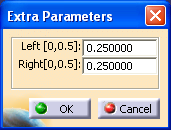
Trapezoid: This distribution creates a trapezoid-shaped curve. Two Extra Parameters are needed for this distribution. They control the percent of the total range that will be in each triangular portion of the distribution.
Notes:
•Clicking on the Trapezoid button, the Extra Parameters dialog box opens displaying Left and Right parameters. Using this dialog box the distribution can be customized as needed.
•When using a Trapezoid distribution, entering a side that is skewed to a larger distribution is allowed, however, the sum of the Left and Right sides must be less than 1. If it equals 1 then the distribution becomes Triangular.
•The Extra Parameters can also be modified when exporting to Excel. The new settings will be imported back in 3DCS, and update the Trapezoid distribution.
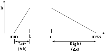
Left parameter represents the length of the "growing" section, and Right parameter represent the length of the "decaying" section, for a standard distribution with a range of one. These parameters should vary within [0, 0.5] interval. The b, c, and h values for the user distribution will be calculated based on the Left (Db), Right (Dc), min and max values, as follows:
parameter_1= Δb / (max-min)
parameter_2= Δc / (max-min)
parameter_1 + parameter_2 < 1.
***It is a triangular distribution when parameter_1 + parameter_2 = 1.
DE Focus Article: Issue 29 - Trapezoidal Distribution - Simulated Distribution in 3DCS
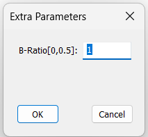
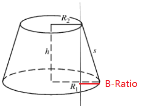
Trapezoid-2D: The resultant shape for the samples is a truncated cone; the samples distribution is equally likely for small radius, a decreasing likelihood (r) for larger radii, and trapezoidal shape through any angle.
For this Trapezoid-2D distribution the Extra Parameters will be represented by one value, B-Ratio, since the distribution is symmetrical.
Power Function: The Power Function Distribution (PFD) is a flexible distribution as it is able to model the various types of data. It is usually used for the reliability analysis, life time and income distribution data.
Power function distribution formula is:
f(x) = cx^(c-1)/b^c
The range for x is between zero and b: 0 <= x <= b
c is the shape parameter. The default value for c is 0.5
b is the Range value from the tolerance dialog.