3DCS includes different methods of model analysis. Although each method has pro's and con's, all Analysis methods are widely accepted methods of dimensional analysis. For more information on these analysis, please see the Monte Carlo analysis, Contributor Analysis, or Analysis Comparison & Assumptions sections. For more information about Linearity please see the Univariate Linearity Percentage article published in the DE news, available on the Community website.
The purpose of this section is to explain how the terms linear and non-linear apply to a 3DCS model and how they affect the analysis. This section also includes methods for determining the amount of non-linearity in a model. |
Part 1
A 3DCS model is a model of the relationships between variation inputs (tolerances) and variation outputs (measures.)
A simple model is shown below. The measure has a 1:1 relationship with the tolerance. In equation form:
Measure = 1 * Tolerance deviation + basic dimension
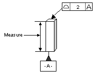
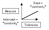
This is an example of the simplest relationship, a linear relationship. In general form, the relationship is:
Measure = constant1 * tolerance + constant2
If this relationship were graphed, it would form a line.
A model with multiple tolerances is still linear if each tolerance has a linear relationship with the measure, such as:
Measure = A * (tol1) + B * (tol2) + C * (tol3) … + N * (toln) + constant
Each tolerance must be to the power of one for the relationship to be linear. The relationship shown below is non-linear.
Measure = A * (tol1) + B * (tol1)2
Furthermore, each tolerance must have an independent relationship with the measure, so that the value of one tolerance does not change the relationship of another. The following equation is not linear, since the tolerances interact (different values for tol2 will change the relationship between Measure and tol1.)
Measure = A * (tol1) + B * (tol1) * (tol2)
The tolerances can also interact if a discontinuity exists in the relationship between the measure and the tolerances. For example:
Measure1 = A * (tol1) + B * (tol2)
If Measure1 > C, then Measure2 = D * (tol1) + E * (tol2)
If Measure1 < C, then Measure2 = F * (tol1) + G * (tol2)
While Measure1 is linear, Measure2 is non-linear.
Part 2
By using Monte Carlo analysis, 3DCS can model both linear and non-linear relationships between the inputs and outputs. For example, a 3DCS model with two tolerances could be created with the following relationship:
Measure = A * (tol1) + B * (tol2) + C * (tol1)2 + D * (tol1) * (tol2)
The HLM and GeoFactor analysis, however, cannot completely analyze this relationship because it is non-linear. Both of these tools analyze the model by varying a single tolerance at a time. All other tolerances are left at nominal (zero deviation). Therefore, any tolerance interactions, such as in the last term above, are not analyzed since the result of the term will be zero. Furthermore, each of these tools picks two points at which it compares the relationship between measure and tolerance at two points. These two points can define one linear relationship or infinite non-linear relationships. The calculations of the two tools assume the linear relationship. These results are always valid under the conditions of the analysis, however their use will differ. In a linear model, eliminating a 50% contributor will always reduce the measure variation by 29.3%. In a non-linear model, the Simulation must be re-run to determine the effect.
A 3DCS model is linear on a measure-by-measure basis, i.e., a model can contain both linear and non-linear measures. The following is a partial list of possible causes of non-linearity in a measure:
1) The measure measures variation along multiple directions.
E.g., True Distance Mode measures a point along infinite directions
2) The measure measures angular variation (variation along an arc) along a vector.
3) The measure measures non-angular variation with an Angle measure.
4) The measure includes logic, such as finding the minimum value of a set of measures.
5) A vector in the moves, measures or tolerances is dynamic (e.g. Two Pt Type).
6) The moves include Conditional Logic, Iterative (Interference) Logic, R-Touch moves, Iteration moves, Pattern moves, Gravity moves, or Plane-Plane moves.
7) The moves include a User-DLL or User-Defined moves that introduces non-linearity.
8) An Object-Target pair in a move is rotated more than 45º relative to each other after tolerances are applied.
7) Either object features or target features can vary so much that their relative positions can switch.
8) Dual, Triple, User-DLL or User-Defined tolerances are used.
9) The model contains size tolerances and either hole-pin floating or bonus
tolerance (MMC modifiers).
These conditions are not sufficient for measuring non-linearity. The relationship between the measure and the tolerances is what truly determines non-linearity. 3DCS is often used to model complex 3-dimensional assemblies. Therefore, very few measures will be completely linear. 3DCS includes extra calculations in the HLM and GeoFactor analyses to capture the effects of two common sources of non-linearity: bonus tolerance and the interaction of size tolerance and hole-pin float.
Although most measures are non-linear, most of these measures are effectively linear. Consider the following geometry:
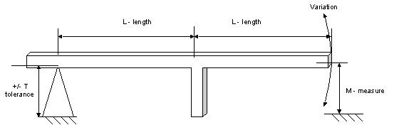
The relationship between the tolerance deviation and the measure is:
M = L * sin( arctan( T / L ) )
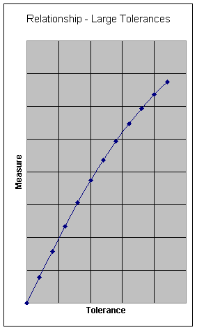
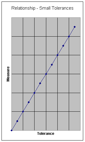
As can be seen on the left hand graph below, this relationship is not linear. If the tolerance values are small compared to the length, however, the relationship will become effectively linear. This occurs because if (T / L) Þ 0, sin( arctan (T / L) ) Þ (T / L) and the relationship simplifies to the linear equation M = T.
A practical method to determine if a measure is non-linear is to compare the results of the analyses at different tolerance levels.
For measures in a simple model with tolerances larger than 0.2 mm or 0.2 degrees:
Run a GeoFactor analysis. Compare the 6 sigma results to the Simulation results. If they are similar the model is linear. If they are not similar, either the model is not linear or it is more complex than GeoFactor allows.
For measures in a more complex model with small contributions from Pattern moves or size tolerances:
Run the Contributor Analysis analysis and save the results. Then scale all the tolerances in the model except size tolerances. Also scale all the hole-pin floats. A scale value of 0.1-0.5 will probably work best. Run the Contributor Analysis analysis again and compare the results. Changes in the contributions indicate non-linearity.
For measures in the most complex models:
Run the Simulation analysis and save the results. Then scale all the tolerances in the model including size tolerances. Also scale all the hole-pin floats. A scale value of 0.1-0.5 will probably work best. Run the Simulation analysis again and compare the results. If a measure result is multiplied by the scale value, then it is linear.