The Monte Carlo analysis displays all the statistical data of the each measure associated in an assembly. A statistical report for each measurement is generated. A detailed description of each of the output parameters in the report is outlined below.
|
Analysis Summary |
Monte Carlo (Histogram) and the Contributor Results |
|
|
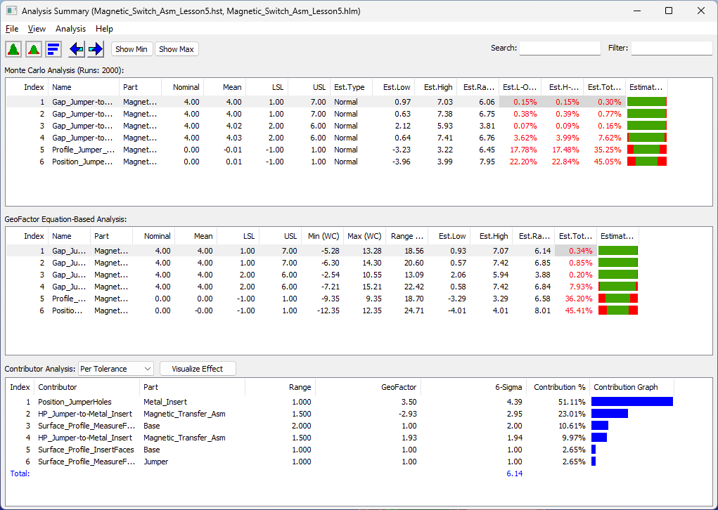
The Analysis Summary shows all the measures and the Contributors that affect the measures results. Double-click on one of the measures in the list to see the Monte Carlo results in a Histogram.. |
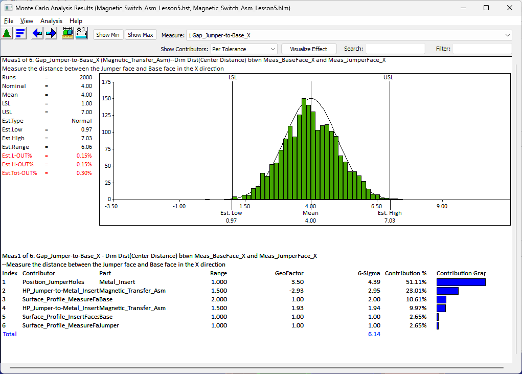
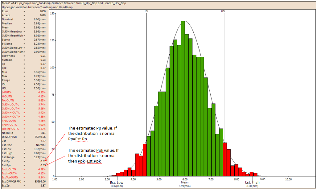
The Monte Carlo results (Histogram) shows the statistical results of the measure. The Contributor Analysis can also be shown or hidden. |
Complete Process Report
Histogram
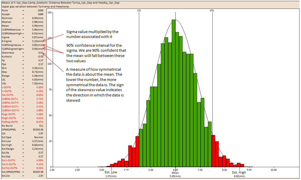
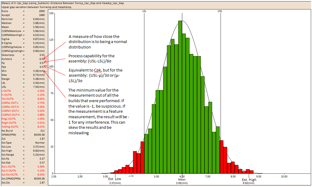
The histogram is a type of bar graph that plots frequency distributions. The histogram consists of bars that represent the complete range of the data. Each bar has a high and a low limit. Each measurement value, generated by the simulation, is assigned to the bar within whose range it falls in. The height of the bar represents the number of measurement values within it. A histogram is generated for each measurement of the assembly model.
Frequency
The frequency of measurements that fall in the range of a particular bar of the histogram.
The Upper Spec. Limit (USL) and the Lower Spec. Limit (LSL) are displayed as two lines on the histogram. The histogram bars outside the USL and LSL may be denoted in a different color signifying that they are out of range. If the spec limits are very large as compared to the simulated data distribution, the histogram does not display the spec limits.
The histogram's Est Low and Est High from the Mean values are displayed on either side of the Mean value.
A detailed description of all the statistical data is given below: Type, Measure, Runs, Nom., Mean, Sigma, Min, Max., Range, CP, CPK, LSL, USL, L-Out, R-Out and Curve Fit associated with the histogram.
Name: Displays the name given to identify the measurement. Example: MEAS1(default), Upper Gap etc.
Type: The top section of the process report contains the Type of measurement. It displays the type of measurement used for that particular output. Example: Pt. Distance, Line Angle etc.
Description: Displays the measurement description as shown in the measurement dialog box. Example: Distance Between TurnLP_Upr_Gap and HeadLP_Upr_Gap.
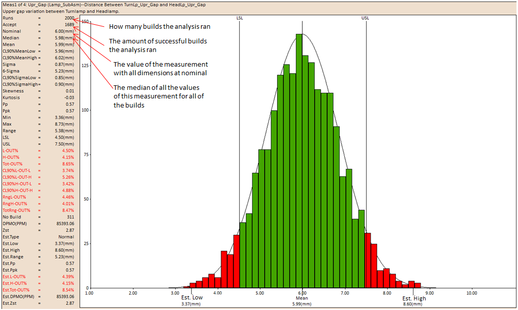
No Builds: Displays the amount of builds that failed to build.
Runs: This is the actual number of Monte Carlo simulation runs that have been performed on the assembly build.
Nominal
The Nominal value of the measurement is the value when all tolerances associated with the measurement are at their nominal values and all moves have been performed.
Accept
Accept represents the number of accepted builds, and is calculated as the difference between the Total Runs and Calculated Failed Assemblies.
Note: The example below shows the relationship between Total Runs, Calculated statistics for No Builds, Runs and Accept:
Total Runs = 2000
No Builds = 5
Case 1: Calculated statistics for No Builds option is checked => Runs = 2000; Accept = 1995
Case 2: Calculated statistics for No Builds option is not checked => Runs = 1995; Accept = 1995
Median: The median value of the simulated data.
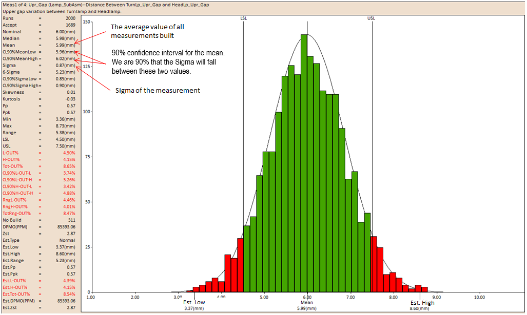
Mean: The mean or average value of the population generated by the process simulation.
CLnn%MeanLow/CLnn%MeanHigh
The nn% confidence interval for the mean, assuming that the data is normally distributed.
Note: nn denote the value from 0 to 99%
Sigma: STD denotes Standard Deviation which is a statistical measure of variation:

6-Sigma
It is the Standard Deviation value multiplied by the number used in the Sigma Number. This represents the width of the normal curve.
The Sigma Number in the Analysis Options controls the STD number. With 6 Sigma Number (+/-3) the Estimated Percent will equal 99.73%. Changing the Sigma Number will change the Estimated Percent. For example: changing the Sigma Number to 12 Sigma (+/-6) will equal 99.999%, which will change the Estimate High, Estimated Low and Estimated Range values.
CLnn%STD-Low/CLnn%STD-High
The nn% confidence interval for the standard deviation, assuming that the data is normally distributed.
Note: nn denote the value from 0 to 99%
Skewness
The Skewness of the simulated data.
Kurtosis
The Kurtosis of the simulated data.
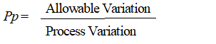
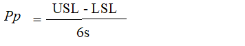
Pp
Pp is a Process Performance index which measures the performance of the process. This index compares the variation of the process to the allowable variation that is set by the specification limits (USL and LSL).
Process Performance index, Pp, is similar to Process Capability index, Cp. Outside of the context of Statistical Process Control (SPC) there is no difference between Cp and Pp, and only the term Cp is used. When sample data is in view, s is estimated by the familiar sample standard deviation that is technically denoted as s.
It is within the context of SPC that the distinction between Cp and Pp becomes important. The difference is in the estimate of s that is used. In SPC, measurements are collected in subgroups.
For Cp, s is estimated by 2 / d2 , which is the average range of the subgroups divided by a scale factor called d2 that is dependent on the subgroup size. For Pp, s is estimated by s. Since 3DCS does not record measurements in numerous small subgroups, but rather one large group, Pp is more appropriate to use.
The Pp index tells us about the capability of a process but does not tell us where the process lies with respect to its center.
When the range between the Upper Design Limit (UDL) and Lower Design Limit (LDL) is the same as the 6 sigma spread, the Cp index will be 1.0.
The Pp index is calculated for a bilateral tolerance, there is no universally accepted way of defining Pp Index for a unilateral tolerance.
Controlling Factors for Cp:
Design Specifications
Standard Deviation
Sources of the Deviation
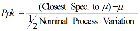
Ppk
The Ppk indicator is a Process Performance index which tells us how well the process is centered, or how distant the mean of the process is compared to its specification limit. The Ppk index can never be higher than the Pp index value. If the Ppk and Pp values are equal, the process is centered. If the Ppk value is 0, the mean of the process is centered about one of its specification limits.
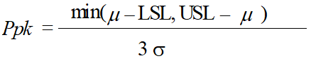
Where:
min = Minimum Value
m = Mean Value
s = Standard Deviation
Controlling Factors for Ppk:
Design Specifications
Standard Deviation
Sources of the Deviation
Central tendency of Process
Minimum (Min): The minimum value of the measurement generated during a given set of process simulations for that particular measurement.
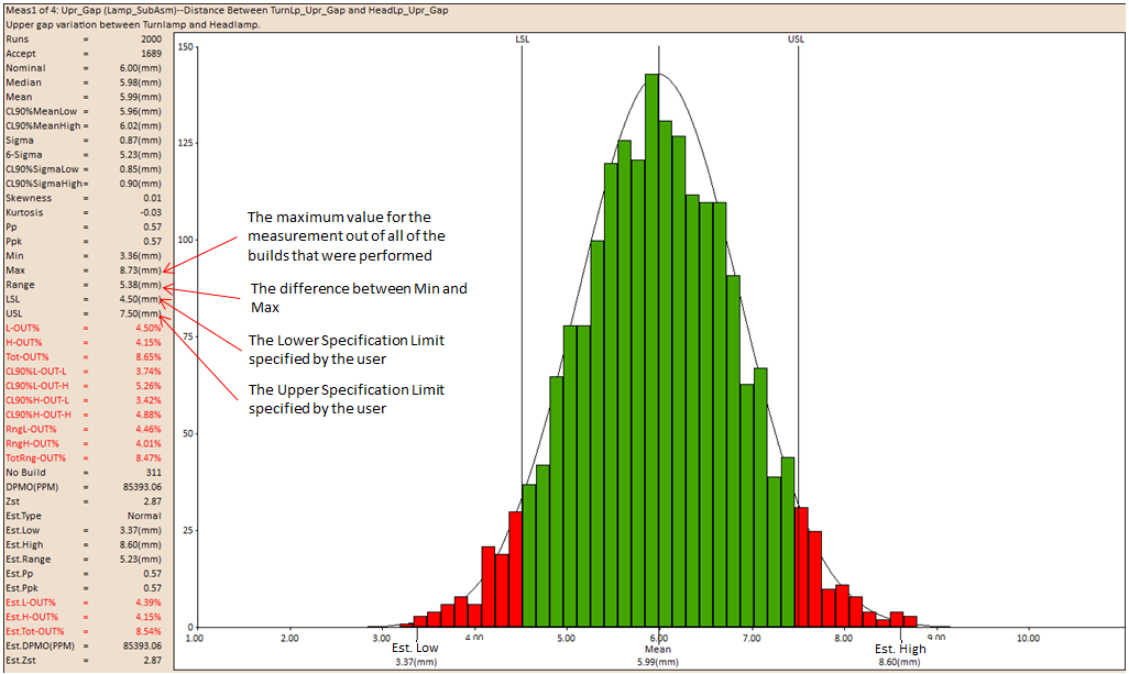
Max: Max is the maximum value of the measurement generated during a given set of process simulations for that particular measurement.
Range: The difference between the maximum value and the minimum value constitutes the range.
LSL: LSL is the Lower Specification Limit number set for that particular measurement.
USL: USL is the Upper Specification Limit number set for that particular measurement.
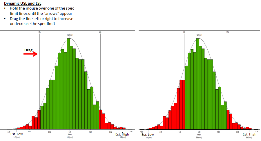
Note: The LSL and USL can be dynamically adjusted, to modify the percent out of spec.
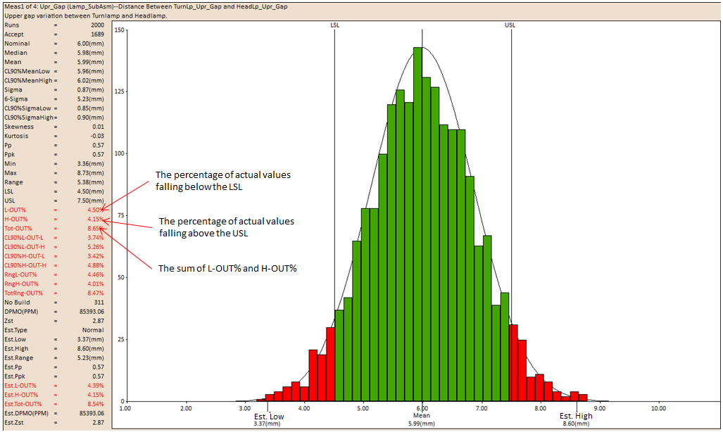
L-OUT%
L-Out is the actual percentage of measurement values falling below the Lower Specification Limit.
H-OUT%
H-Out is the actual percentage of measurement values falling above the Upper Specification Limit.
Tot-OUT%
Tot-OUT% is the actual percentage of measurement values falling above the Upper Specification Limit and below the Lower Specification Limit.
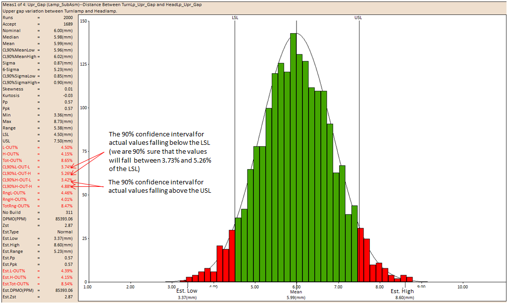
CL90%L-OUT-L / CL90%L-OUT-H
The Confidence Interval for the L-OUT%.
Note: nn denote the value from 0 to 99%
CLnn%H-OUT-L / CL90%H-OUT-H
The Confidence Interval for the H-OUT%.
Note: nn denote the value from 0 to 99%
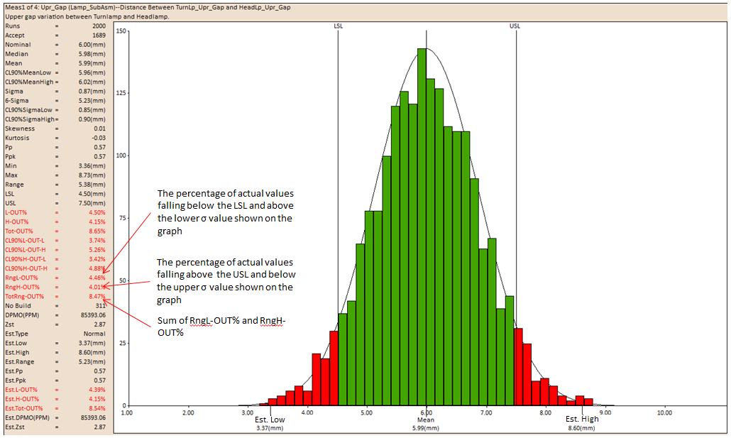
RngL-OUT
RngL-OUT is the actual percentage of statistical measurement values that fall between the Lower Specification Limit and -3STD.
RngH-OUT
RngH-OUT is the actual percentage of statistical measurement values that fall between the Upper Specification Limit and +3STD.
TotRng-OUT
TotRng-OUT is the actual percentage of statistical measurement values that fall between the Lower Specification Limit and -3STD and the Upper Specification Limit and +3STD.
No Build: Number of runs that failed to build.
DPMO(PPM): Defect Parts Per Million: The objective in a Six-Sigma program is to control the production/service process within a 3.4 DPMO. DPMO is directly related with the probability of outside-specification samples. See DE News Issue 55 for more information.
It is important to note that a Normal (Gaussian) distribution is assumed when calculating DPMO in a Six-Sigma program. |

Zst: is used as a checking measurement for a process capability.
•Zst = Z-bench + Z-shift.
•Z-bench: is the Z-score that corresponds to the total probability of a defect.
•Z-score: A quantity in a standard normal distribution (mean µ = 0 and standard deviation s = 1) for a specified probability. For a non-standard distribution, Zscore = (x - µ)/s, where x is a sample value.
•Z-shift: is a shift value for the Z-score. In Six Sigma, Z-shift is usually assumed to be 1.5. (See Preferences to set or change the default).
•See DE New Issue 16 and Issue 55 for more information.
Est Type: Samples are tested for normality. If the sample is determined to be non normal, then the curve fitting function picks the distribution curve that best fits the data set. There are seven alternative curve fits: Constant, Min-Max, and Pearson I, III, IV, V or VI.
Normality tests fail for large sample sizes even if the underlying distribution is normal [1,2]. As the sample size grows, the probability of values in the tails increases. These large values cause the normality tests to fail.
Therefore, 3DCS uses 2000 as the maximum number of samples in the normality test. The statistics are calculated using ALL the samples. Only the number of samples is changed in the normality test.
1.Arnastauskaitė J, Ruzgas T, Bražėnas M. An Exhaustive Power Comparison of Normality Tests. Mathematics. 2021; 9(7):788.
2.Mohd Razali, . Nornadiah et al Power comparisons of Shapiro-Wilk, Kolmogorov-Smirnov, Lilliefors and Anderson-Darling Tests. Journal of Statistical Modeling and Analytics. Vol.2 No.I, 21-33, 2011
3.Robert Greener Stop testing for normality. Towards Data Science; 2021
.
Curve Fit Information

Est.Low: For the Normal and Pearson curves the Estimated Low is selected so that .135% of the area under the curve is in the lower tail.
Est.High: For the Normal and Pearson curves the Estimated High is selected so that .135% of the area under the curve is in the upper tail.
Est.Range: The Estimated Range is the difference between the Estimated High and Low values. In the case of the Normal curve, this range corresponds to +/- 3 sigma interval.

Estimated Pp
Ppest = (USL-LSL)/( X99,865 - X 0,135)
Where X 99,865 is the value 99.865% of the population is estimated to be below and X 0,135 is the value 99.865% of the population is predicted to be above.given the distribution.
When the range between the Upper Design Limit (UDL) and Lower Design Limit (LDL) is the same as the 6 sigma spread, the Cp index will be 1.0.
If the distribution is Normal, then Pp =Ppest.
Estimated Ppk
Ppkest = min [ (USL-μ)/( X 99,865 - μ ) , (μ - LSL)/(μ - X 0,135 )]
Where Min is the minimum value; μ is the mean value
X 99,865 is the value 99.865% of the population is estimated to be below given the distribution.
X 0,135 is the value 99.865% of the population is predicted to be above.given the distribution.
When the range between the Upper Design Limit (UDL) and Lower Design Limit (LDL) is the same as the 6 sigma spread, the Cp index will be 1.0.
If the distribution is Normal, then Ppk =Ppkest.
Est.L-OUT%: The Estimated Low Percentage Out of Spec is the percentage of the estimated curve that falls below the specified Lower Spec. Limit.
Est.H-OUT%: The Estimated High Percentage Out of Spec is the percentage of the estimated curve that falls above the specified Upper Spec. Limit.
Est.Tot-OUT%: The Estimated Total Percentage Out of Spec is the percentage of the estimated curve that falls below the specified Lower Spec. Limit and that falls above the specified Upper Spec. Limit.

Est.DPMO(PPM): PPM – defect Parts Per Million calculated from the curve fit. This value corresponds with Est.Tot-OUT% and is interchangeable with DPMO – Defects Per Million Opportunities
Est.Zst: Represents the process capability. Usually, Zst equals to Z-bench + Z-shift.
•Z-bench - is the Z-score that corresponds to the total probability of a defect.
•Z-score – For a non-standard distribution, Zscore = (x - µ)/s, where x is a sample value.
•Z-shift – is a shift value for the Z-score. In Six Sigma, Z-shift is usually assumed to be 1.5.

This value that should be used when comparing the 3DCS model output to GD&T on a drawing or determine what value to use in the Feature Control Frame on the drawing. It is the size of the zone that contains the percent of samples specified by the Sigma Number (±3σ). To put it another way, Recommended GD&T Value reports the predicted variation in terms of GD&T standards.
Recommended GD&T Value only applies to GD&T Measure types. All other types will show "N/A" for this value.
Recommended GD&T Value is calculated using a simple equation that will take variation and mean shift into account:by: 2*max(abs(Est.Lowi), Est.Highi)
![]()
where i is the index of a feature in the Features List and Max is the maximum between the two values.
Recommended GD&T Value outputs a value that is centered at the nominal. Mean shifts will increase the Recommended GD&T Value regardless of the range of variation.
For example, if one GD&T Measure returns
Nominal = 0
Mean = 0
Est.Low = -0.5
Est.High = 0.5
Est.Range = 1
then:
![]()
In this case, |Est.Low| = Est.High so the max is 0.5 either way.
Now if another GD&T Measure returns
Nominal = 0
Mean = -0.25
Est.Low = -0.75
Est.High = 0.25
Est.Range = 1
then
![]()
Notice how the second measurement has a larger Recommended GD&T Value than the first even though they have the same Est.Range. This is due to the Mean Shift.